Download Unit Tangent, Normal/Binormal Vectors Osculating Plane Acceleration | MTH 254 and more Study notes Calculus in PDF only on Docsity!
Osculating Plane, Acceleration components
If we think of the function r t ( )
G
as describing a particle moving along a curve, then the unit
tangent vector to the function r t ( )
G
when 0
t = t is the unit vector that points in the precise
direction the particle is moving at 0
t = t ; this vector is denoted as ( )
0
T t This idea is most easily
understood when the motion is confined to a plane.
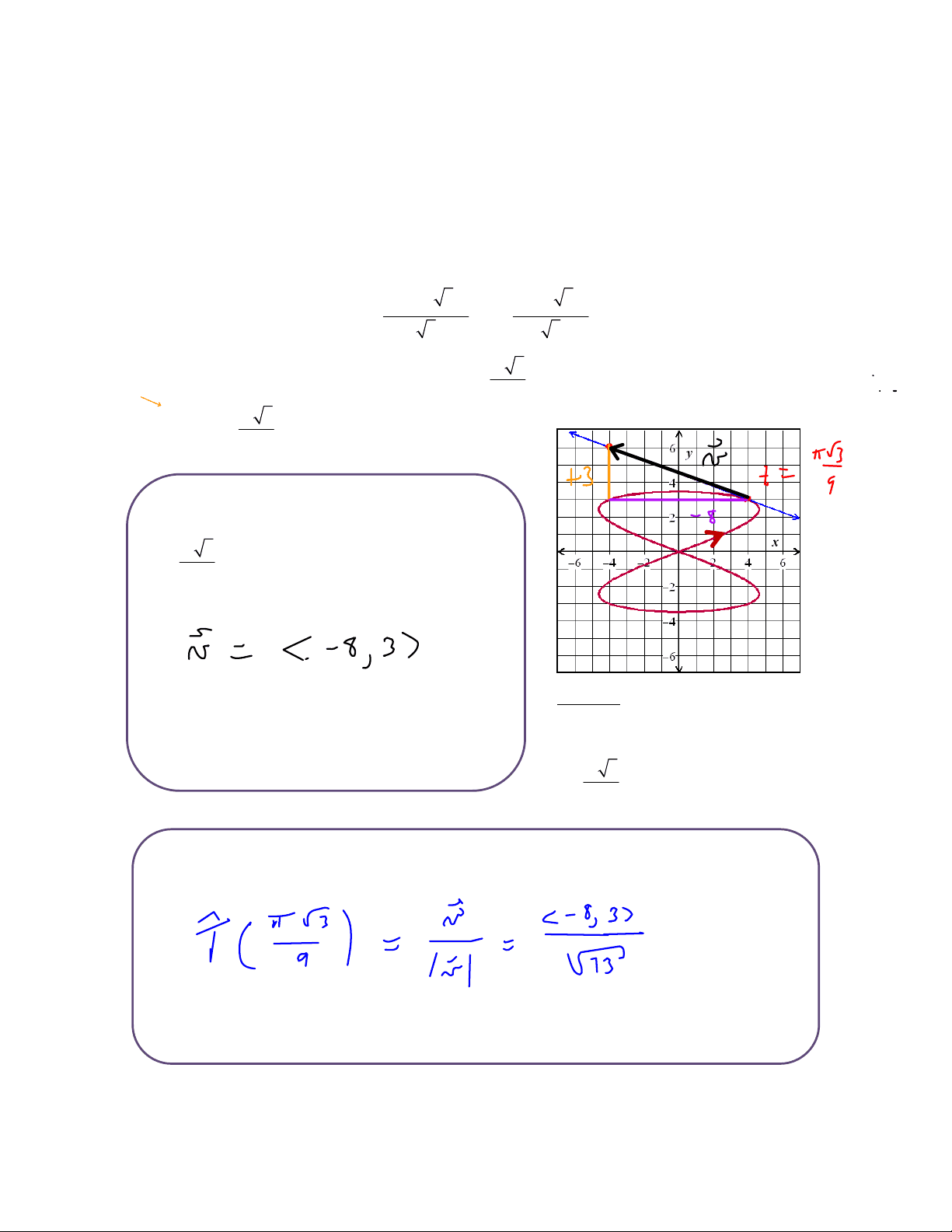
A graph of the function ( )
8sin 2 3 6sin 3
t t
r t i j
G
is shown in Figure 1. The
tangent line to the curve at the point where
t
= is also shown. Let’s use the figure to
determine
T
π
.
Now we need to normalize our direction vector.
The first thing we must determine is any vector
that points in the direction of motion at
t
Figure 1
Tangent line and unit normal
vector to r t ( )
G
at the point where
t
π
Osculating Plane, Acceleration components
Let’s now use the formula ( )
8sin 2( 3 ) 6sin ( 3 )
t t
r t i j
G
to determine
T
.
Let’s be brave and do so by hand.
The first thing we must determine is any vector that points in the direction of motion at
t
Now we need to normalize our direction vector.
Osculating Plane, Acceleration components
( )
( )
( )
0
0
0
T t
N t
T t
; i.e. (^) ( ) 0
N t is the unit
vector in the same direction as ( ) 0
T ′ t.
( )
( )
( )
0
0
0
r t
T t
r t
G
G
; i.e. (^) ( ) 0
T t is the unit
vector in the same direction as (^) ( ) 0
r ′ t
G
Find
T
⎛ (^) π ⎞
.
Store the formula for
r (^) ( ) t
G
as y (^) ( t (^) ).
Find the formula for (^) ( )
T t
and store is as z t ( (^) ).
Verify the formula for (^) ( )
T t
by calculating
z
π
.
Find
N
⎛ (^) π ⎞
.
By definition, (^) ( )
( )
( )
0
0
0
T t
N t
T t
. Let’s use our calculators to find
N
π
.
Osculating Plane, Acceleration components
By definition, the unit binormal vector , (^) ( ) 0
B t
G
, to
r t ( )
G
at 0
t = t is (^) ( ) ( ) 0 0
T t × N t. Let’s draw onto
Figure 1 vectors indicating the directions of
T
π
and
N
⎛ (^) π ⎞
and use the right-hand-
rule to help discern
B
⎛ (^) π ⎞
.
Figure 1
Tangent line and unit normal vector to
r (^) ( t )
G
at the point where
t
π
Let’s “calculate”
B
.
Let’s “calculate”
r
⎛ (^) π ⎞
G
and indicate its
general direction on Figure 1.
What does the position of
r
⎛ (^) π ⎞
G
relative to
T
⎛ (^) π ⎞
and
N
⎛ (^) π ⎞
tell us about the
motion along r t ( )
G
at
t
π
Osculating Plane, Acceleration components
Numerically, we quantify the position and effect of the acceleration vector by the tangential and
normal components of acceleration , (^) ( ) T 0
a t and (^) ( ) N 0
a t.
We leave it to the reader to verify that a formula for the tangential component of acceleration is
( )
( ) ( )
( )
0 0
0
0
T
r t r t
a t
r t
G
G
and that a formula for the normal component of acceleration is
( )
( ) ( )
( )
0 0
0
0
N
r t r t
a t
r t
′ × ′′
G
G
.
If (^) ( ) 0
r ′′ t
G
points in the direction of
this quadrant …
( ) 0
T t
( ) 0
N t
If (^) ( ) 0
r ′′ t
G
points in the direction of
this quadrant …
If (^) ( ) 0
r ′′ t
G
points in the
direction of (^) ( ) 0
− T t …
If (^) ( ) 0
r ′′ t
G
points in the
direction of (^) ( ) 0
N t …
If (^) ( ) 0
r ′′ t
G
points in the
direction of (^) ( ) 0
T t …
Let’s show that ( ) 0 N
a t = ∀ t for the linear function ( ) 0 0
r t = x + a t y , + b t
G
.
Osculating Plane, Acceleration components
Figure 2 shows the function (^) ( ) ( ) ( )
2 2
r t = 4, sin t , cos t
G
along with its unit normal vector, unit
tangent vector, and acceleration vector at
t
Plane: x = 4
Figure 2
Let’s use our calculator to verify the
acceleration vector.
Let’s use our calculator to find the components of acceleration and illustrate the
components on Figure 2.
Let’s find the instantaneous rat e of change in the speed at
t
=. What do we observe?
see next page for
calculator screens
Osculating Plane, Acceleration components
Figure 3 shows a graph of the vector function r (^) ( t (^) ) = 2 + cos (^) ( ) t (^) , 4 + 2 cos (^) ( ) t (^) , 3 +2 sin( ) t
G
in its
osculating plane.
What is the equation of the osculating
plane?
Let’s use Figure 3 to help us discern
T
⎛ π⎞
,
N
⎛ π⎞
,
B
⎛ π⎞
.
Figure 3
Osculating Plane, Acceleration components
Let’s use our calculator to verify
T
,
N
,
B
.
As we illustrated on Figure 3, the osculating plane to (^) r ( t )
G
at
t
= is perpendicular to
B
. Let’s use classic techniques to confirm the equation of the osculating plane.