Docsity
Docsity

Prepare for your exams

Study with the several resources on Docsity


Earn points to download

Earn points by helping other students or get them with a premium plan


Guidelines and tips
Guidelines and tips

MATH 203 Test 2 Solutions: Statistical Inference and Hypothesis Testing - Prof. David K. N, Exams of Statistics

Solutions to test 2 of math 203, focusing on statistical inference and hypothesis testing. Topics covered include z-tests, t-tests, confidence intervals, and margin of error calculations.

Typology: Exams

Pre 2010

Uploaded on 08/18/2009

koofers-user-oqt
koofers-user-oqt ๐Ÿ‡บ๐Ÿ‡ธ

10 documents

1 / 4

Toggle sidebar

This page cannot be seen from the preview

Don't miss anything!

bg1
MATH 203 Test 2 Review Solutions
1. (a) The average lifetime of Type 1 batteries is from 1.55 hours less to 0.86 hours more
than average lifetime of Type 2 batteries. (b) It is not conclusive which type of battery
has the longer average lifetime.
______________________________________________________________________________
2. (a) Re-write the interval as 0.024 โ‰ค p
2
โ€“ p
1
โ‰ค 0.052 and say
The percentage of patients for whom Treatment B worsens the condition is from 2.4
percentage points higher to 5.2 percentage points higher than the percentage of patients
under Treatment A.
(Without re-writing the interval: The percentage of patients for whom Treatment A
worsens the condition is from 5.2 percentage points lower to 2.4 percentage points lower
than the percentage of patients under Treatment B.)
(b) It is clear that Treatment B has the higher percentage of patients with a worsening
of the condition.
______________________________________________________________________________
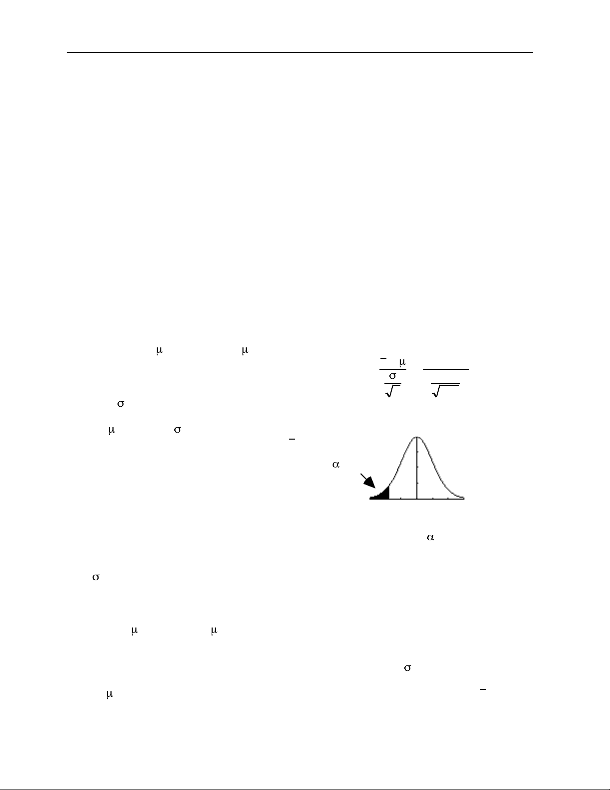
3. (a) Test H0: = 25 vs. Ha: < 25
(b) We can use a Zโ€“Test because the
measurement is normally distributed
and = 2 is known.
(c)
z
= x โˆ’
n
= 24.2 โˆ’25
2
400
= โ€“8
(d) If = 25 and = 2 were true, then
there would be no chance of getting an
x
of 24.2 or lower with a sample of 400 cars.
We can reject H0.
(f) Because we have a large sample, we can
still use the Zโ€“Test even if the
measurement were not normally
distributed. Also, because of the large
sample, we can use
S
as an approximation
for and still use the Zโ€“Test.
โ€“1.645
N(0, 1)
(e)
=0.05
curve
Use โ€“1.96 for
=0.025
.
โ€“โ€“โ€“โ€“โ€“โ€“โ€“โ€“โ€“โ€“โ€“โ€“โ€“โ€“โ€“โ€“โ€“โ€“โ€“โ€“โ€“โ€“โ€“โ€“โ€“โ€“โ€“โ€“โ€“โ€“โ€“โ€“โ€“โ€“โ€“โ€“โ€“โ€“โ€“โ€“โ€“โ€“โ€“โ€“โ€“โ€“โ€“โ€“โ€“โ€“โ€“โ€“โ€“โ€“โ€“โ€“โ€“โ€“โ€“โ€“โ€“โ€“โ€“โ€“โ€“โ€“โ€“โ€“โ€“โ€“โ€“โ€“โ€“โ€“โ€“โ€“โ€“
4. (a) H0: = 6 vs. Ha: > 6 (b) With a small sample, we can use
the Tโ€“Test because the measurement
(birth weight) is normally distributed,
we do not know , but we have S.
(c) If = 6 were true, then there would be an 11.9% chance of getting an
x
of 6.3 or
higher with a sample of size 36. There is not enough evidence to reject H0.
pf3
pf4

Partial preview of the text

Download MATH 203 Test 2 Solutions: Statistical Inference and Hypothesis Testing - Prof. David K. N and more Exams Statistics in PDF only on Docsity!

MATH 203 Test 2 Review Solutions

  1. (a) The average lifetime of Type 1 batteries is from 1.55 hours less to 0.86 hours more than average lifetime of Type 2 batteries. (b) It is not conclusive which type of battery has the longer average lifetime.

  1. (a) Re-write the interval as 0.024 โ‰ค p 2 โ€“ p 1 โ‰ค 0.052 and say

The percentage of patients for whom Treatment B worsens the condition is from 2. percentage points higher to 5.2 percentage points higher than the percentage of patients under Treatment A.

(Without re-writing the interval: The percentage of patients for whom Treatment A worsens the condition is from 5.2 percentage points lower to 2.4 percentage points lower than the percentage of patients under Treatment B.)

(b) It is clear that Treatment B has the higher percentage of patients with a worsening of the condition.


  1. (a) Test H 0 : = 25 vs. Ha : < 25

(b) We can use a Zโ€“Test because the measurement is normally distributed and = 2 is known.

(c) z =

x โˆ’

n

(d) If = 25 and = 2 were true, then there would be no chance of getting an x of 24.2 or lower with a sample of 400 cars. We can reject H 0.

(f) Because we have a large sample , we can still use the Zโ€“Test even if the measurement were not normally distributed. Also, because of the large sample, we can use S as an approximation for and still use the Zโ€“Test.

โ€“1.

N (0, 1)

(e)

= 0.

curve

Use โ€“1.96 for = 0..

  1. (a) H 0 : = 6 vs. Ha : > 6 (b)^ With a small sample, we can use the Tโ€“Test because the measurement (birth weight) is normally distributed, we do not know , but we have S.

(c) If = 6 were true, then there would be an 11.9% chance of getting an x of 6.3 or

higher with a sample of size 36. There is not enough evidence to reject H 0.

(d) n = 36, use t (35) curve

(e) t =

x โˆ’ S n

The test stat of 1.2 is not in the rejection region beyond 1.690; so x is not too large and there is not enough evidence to reject H 0.

  1. Here p = 0.

(a) Test H 0 : p = 0.60 vs. Ha : p > 0.

(b) z =

p โˆ’ p p ร— (1 โˆ’ p ) n

0.60 ร— 0.

= 1.9365 (^) (c) 1.

N (0, 1)

curve

Use 1.96 for a 2.5% level of significance.

(d) If p = 0.60 were true, then there would be only a 2.64% chance of obtaining a p of

0.63 or higher with a sample of size 1000. We can reject H 0 because the P -value is less

than 0.05. (Also, the test stat of 1.9365 is in the rejection region beyond 1.645.)

(e) For = 0.025, the test statistic of z = 1.9365 is not in the rejection region beyond 1.96 (so the P -value is more than 0.025). Thus, with a 2.5% level of significance, p = 0. would not be considered too large and we would not have enough evidence to reject H 0.

  1. (a) n โ‰ฅ

z (^) /2 ร— 0. e

2

1.96 ร— 0.

2 = 909.254438 ; a sample of size 910 is required.

(b) n โ‰ฅ

1800 ร— 909.

= 604.322 ; so now we only need a sample of size 605.

______________________________________________________________________________

  1. (a) p =

= 0.36. Then p โ‰ˆ p ยฑ

z (^) /2 p (1โˆ’ p ) n

2.576 ร— 0.36 ร— 0.

0.36 ยฑ 0.04. That is, 0.32 โ‰ค p โ‰ค 0.40. (Can use the 1โ€“PropZInt to compute the confidence interval with this formula.)

With max margin of error: p โ‰ˆ p ยฑ

z (^) /2 ร— 0. n

2.576 ร— 0.

  1. Large samples: Can use the 2โ€“SampZInt here:

By Hand:

1 โˆ’^2 โ‰ˆ^ ( x 1 โˆ’^ x^ 2 )^ ยฑ^ z^ /

S 12

n 1

S 22

n 2

3.8^2

______________________________________________________________________________

(a) Sp =

23 ร— (0.42)^2 + 29 ร— (0.46)^2

(b) Using the 2โ€“SampTInt screen set to Pooled , we obtain โ€“0.5433 โ‰ค 1 โˆ’ 2 โ‰ค โ€“0.

(or 0.0567 โ‰ค 2 โˆ’ 1 โ‰ค 0.5433). That is, the average weight gain for babies on Formula B is from 0.0567 lbs higher to 0.5433 lbs higher than the average weight gain for babies on Formula A.