Docsity
Docsity

Prepare for your exams

Study with the several resources on Docsity


Earn points to download

Earn points by helping other students or get them with a premium plan


Guidelines and tips
Guidelines and tips

Notes on Adaptive Quadrature - Introduction to Scientific Computing | CS 340, Study notes of Computer Science

Material Type: Notes; Professor: McNelis; Class: Intro Scientific Comp; Subject: Computer Science; University: Western Carolina University; Term: Fall 2009;

Typology: Study notes

Pre 2010

Uploaded on 08/16/2009

koofers-user-nto-1
koofers-user-nto-1 🇺🇸

10 documents

1 / 2

Toggle sidebar

This page cannot be seen from the preview

Don't miss anything!

bg1
CS 340 - Introduction to Scientific Computing
Section 5.5: Adaptive Quadrature
The Idea: Using a composite integration technique with different subinterval widths (h) in order to
approximate the value of a definite integral, Rb
af(x)dx, correct to within a certain tolerance, ². Portions
of the f(x) curve with a large variation in values should require much smaller values of h, and portions of
the f(x) curve with little change in y-values would correspond to larger values of h. See the illustration
below.
Larger h−values
Less Variation
Smaller h−values
needed
More Variation
The Concept:
Approximate the integral over the initial interval.
Then approximate the integral over the left and right
half subintervals of that interval.
If the difference in the approximations for the area over
the original interval is less than the tolerance, STOP;
Return the sum of the integral over the two halves.
Otherwise, repeat this process, subdividing each of the new
subintervals.
The Adaptive Quadrature Process (with Simpson’s 1
3Rule and Error Tolerance ²):
Stage 1:
Begin with the initial interval, [a,b]
Define ²1=².
Define S1[a, b] to be the results using Simpson’s 1
3rule with h1=ba
2to approximate Rb
af(x)dx.
Stage 2:
Cut the interval in half.
Define S2ha, a+b
2iand S2ha+b
2, bito be the results of using Simpson’s 1
3rule with h2=h1
2=ba
4
over the left and right half subintervals, respectively.
Test if ¯
¯
¯
¯
S1[a, b]µS2·a, a+b
2¸+S2·a+b
2, b¸¶¯
¯
¯
¯
< ²1
If so, stop your subdividing. Let A2=S2ha, a+b
2i+S2ha+b
2, bibe your final result.
If not, continue this halving process and repeat the same tests on each subinterval with ²2=1
2²1.
.
.
.
pf2

Partial preview of the text

Download Notes on Adaptive Quadrature - Introduction to Scientific Computing | CS 340 and more Study notes Computer Science in PDF only on Docsity!

CS 340 - Introduction to Scientific Computing Section 5.5: Adaptive Quadrature

The Idea: Using a composite integration technique with different subinterval widths (h) in order to approximate the value of a definite integral,

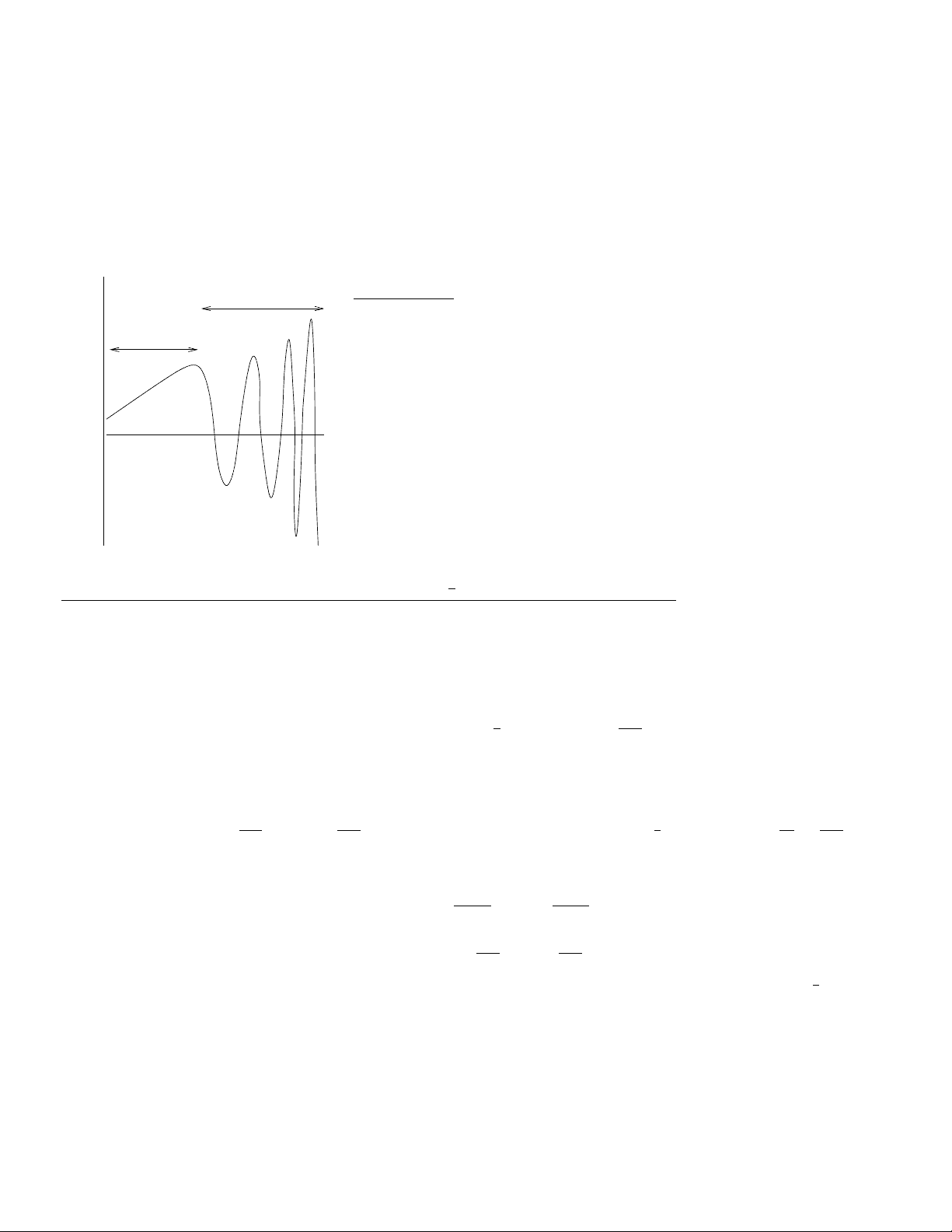
∫ (^) b a f^ (x)^ dx, correct to within a certain tolerance,^ ≤. Portions of the f (x) curve with a large variation in values should require much smaller values of h, and portions of the f (x) curve with little change in y-values would correspond to larger values of h. See the illustration below.

Larger h−values

Less Variation

Smaller h−values needed

More Variation The Concept:

Approximate the integral over the initial interval.

Then approximate the integral over the left and right half subintervals of that interval.

If the difference in the approximations for the area over the original interval is less than the tolerance, STOP; Return the sum of the integral over the two halves.

Otherwise, repeat this process, subdividing each of the new subintervals.

The Adaptive Quadrature Process (with Simpson’s 13 Rule and Error Tolerance ≤):

Stage 1:

  • Begin with the initial interval, [a, b]
  • Define ≤ 1 = ≤.
  • Define S 1 [a, b] to be the results using Simpson’s 13 rule with h 1 = b− 2 a to approximate

∫ (^) b a f^ (x)^ dx.

Stage 2:

  • Cut the interval in half.
  • Define S 2

[ a, a+ 2 b

] and S 2

[ a+b 2 , b

] to be the results of using Simpson’s 13 rule with h 2 = h 21 = b− 4 a over the left and right half subintervals, respectively.

  • Test if (^) ∣ ∣∣ ∣S^1 [a, b]^ −

( S 2

[ a,

a + b 2

]

  • S 2

[ a + b 2

, b

])∣∣ ∣∣ < ≤ 1

  • If so, stop your subdividing. Let A 2 = S 2

[ a, a+ 2 b

]

  • S 2

[ a+b 2 , b

] be your final result.

  • If not, continue this halving process and repeat the same tests on each subinterval with ≤ 2 = 12 ≤ 1. .. .

Stage i:

  • Calculate, Si[ai, bi], the approximation to the area over the ith^ subinterval [ai, bi] using hi = bi−ai 2.
  • Divide that subinterval in half (getting the i+1st^ subintervals) and calculate the area, Si+

[ ai, ai+ 2 bi

]

and Si+

[ ai+bi 2 , bi

] over each half using hi+1 = 12 hi.

  • Check if (^) ∣ ∣∣ ∣Si[ai, bi]^ −

( Si+

[ ai,

ai + bi 2

]

  • Si+

[ ai + bi 2

, bi

])∣∣ ∣∣ < ≤i

  • If YES, stop, and final answer results from A 2 = Si+

[ ai, ai+ 2 bi

]

  • Si+

[ ai+bi 2 , bi

] .

  • If NO, repeat this process on each of the subintervals Si+

[ ai, ai+ 2 bi

] and Si+

[ ai+bi 2 , bi

] sepa- rately with ≤i+1 = 12 ≤i.