Download Multi Step Methods-Numerical Methods in Engineering-Lecture 22 Slides-Civil Engineering and Geological Sciences and more Slides Numerical Methods in Engineering in PDF only on Docsity!
CE 341/441 - Lecture 22 - Fall 2004
p. 22.
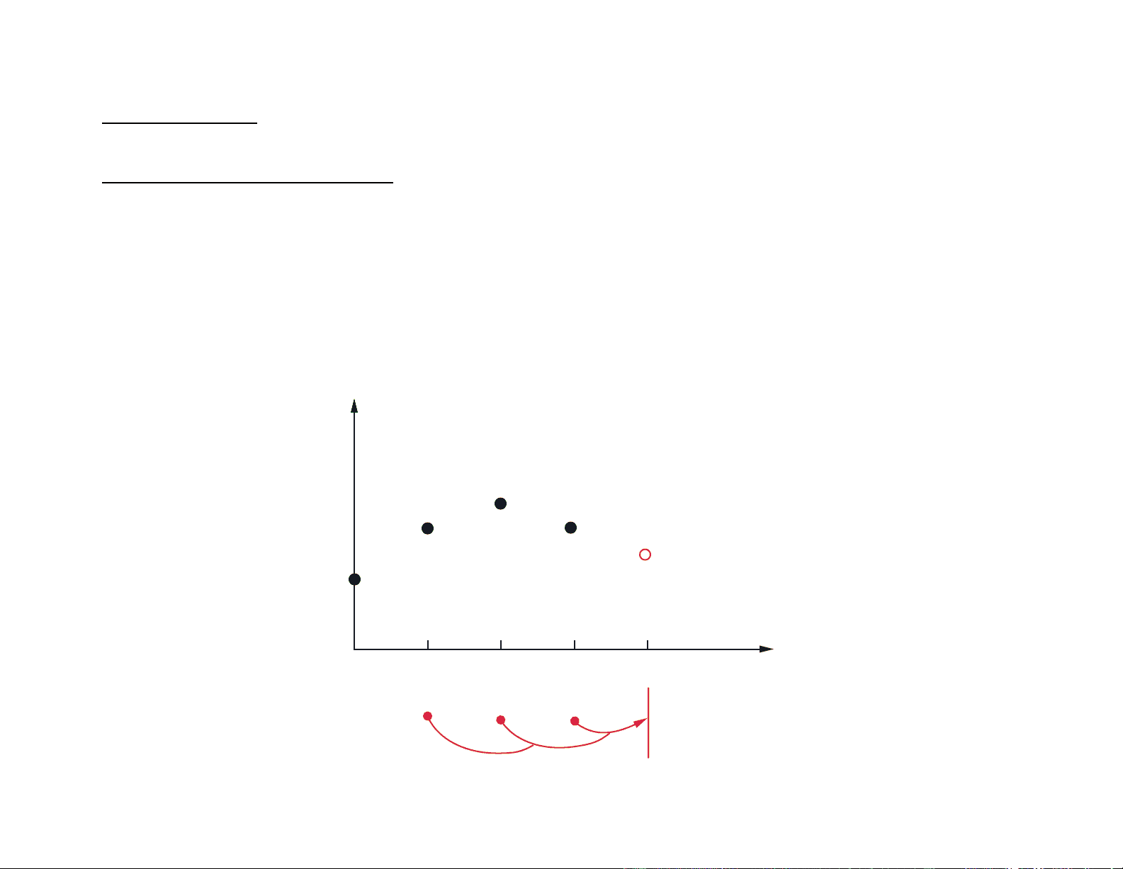
LECTURE 22MULTI STEP METHODS • Solve the i.v.p. • Multi step methods use information from several previous or known time levels^ INSERT FIGURE NO. 100
dy ----- dt
-^
f^
y t ,(
y t
o (^
)^
y^ o
y
t
y^0
t^0
t^1
t^2
t^3
t^4
y^1
y^2
y^3
y^4
CE 341/441 - Lecture 22 - Fall 2004
p. 22.
• Open Formulae (Adams-Bashforth)
• explicit (non-iterative)• can have stability problems
• Closed Formulae (Adams-Moulton)
• implicit (iterative)• much better stability properties than open formulae
• Predictor-Corrector Methods
• 1 cycle predictor
→
open formula
• 2-3 cycles corrector
→
closed formula
• superior to either open or closed formulae separately
CE 341/441 - Lecture 22 - Fall 2004
p. 22.
2nd Order Accurate Adams Open Formula • Use a backward difference approximation for• Substituting we obtain:
⇒
⇒
⇒
˙ f j
˙ f j
f^
j^
f^
j^
1
-^ ∆
t
-^
t 2
˙˙ f j^
O
t (^
y^
j^
1 +^
y^
j^
t^
f^
j
t 2
f^
j^
f^
j^
1
-^ ∆
t
-^
t 2
˙˙ f j^
O
t (^
t (^
-^
˙˙ fj
^
^
^
y^
j^
1 +^
y^
j^
t^
3 ---^2
f^
j
1 ---^2
f^
j^
1
–^
t (^
f
˙˙ j
O
t (^
y^
j^
1 +^
y^
j^
t^
3 ---^2
f^
j
1 ---^2
f^
j^
1
–^
O
t (^
y^
j^
1 +^
y^
j^
t^
3 ---^2
f^
y^
j^
t^ , j
(^
)^
1 ---^2
f^
y^
j^
1
-^
t^ j
1
,
(^
–^
O
t (^
CE 341/441 - Lecture 22 - Fall 2004
p. 22.
INSERT FIGURE NO. 101 • Notes
• Method is second order since the local truncation term is
(recall the effect of
cumulative error during time stepping)
• Formula was derived by developing a forward Taylor series for
about
and
using a backward finite difference approximation for the first derivative of
• Note that the method is
explicit
→
i.e. the new time level
value is computed
using the slope at the current and previous time levels
and
• This formula is
not self starting
! Use 2nd order Runge-Kutta (R.K.) method to start
the computations
y(t)
t
tj-
tj^
tj+
yj-
yj
yj+
O
t (^
y^
j^
1 +^
y^
j f^
y^
j^
t^ , j
(^
j^
j^
j^
CE 341/441 - Lecture 22 - Fall 2004
p. 22.
• From time level
to
; apply 2nd order Adams Open Formula
Now we know
• From time level
to
; apply 2nd order Adams Open Formula
Now we know
j^
j^
t^2
t^1
t
= y^2
y^1
t^
3 ---^2
f^
y^1
t 1 , (^
)^
1 ---^2
f^
y^ o
t o , (^
y^2
t^2 j^
j^
t^3
t^2
t
= y^3
y^2
t^
3 ---^2
f^
y^2
t 2 , (^
)^
1 ---^2
f^
y^1
t 1 , (^
y^3
t^3
CE 341/441 - Lecture 22 - Fall 2004
p. 22.
INSERT FIGURE NO. 102
y(t)
t
y^0
t^0
t^1
t^2
t^3
y^1
y^2
y^3
2nd order R-K
2nd order Adams Open
2nd order Adams Open
*y 1
CE 341/441 - Lecture 22 - Fall 2004
p. 22.
INSERT FIGURE NO. 103A • Method is third order accurate• Need to start this method with 2 steps of a 3rd order accurate R.K. method
• i.c. gives
• R.K. starter gives
,^
and
• Now we can use the 3rd order Adams Open Formula
y(t)
t
tj-
tj-
tj^
tj+
yj-
yj-
yj
yj+
y^ o
t^ o
y^1
t^1
y^2
t^2
CE 341/441 - Lecture 22 - Fall 2004
p. 22.
Summary of Adams Open Formulae • General form of all Adams Open formulae• Formulae are explicit:
is computed in terms of slope at
,^
• All higher order Adams formulae are not self starting (don’t know
,^
, etc.).
• Must start method with an appropriate order Runge-Kutta formula.
• Open formulae are more efficient than R.K. methods of the same order since slope
calculations
at a given point are re-used for at least several time steps.
• Open formulae are very easy to implement• Open formulae
may
have stability problems
y^
j^
1 +^
y^
j^
t^
α
f^
y^
j^
t^ , j
(^
)^
β
f^
y^
j^
1
-^
t^ j
1
,
(^
)^
γ^
f^
y^
j^
2
-^
t^ j
2
,
(^
)^
δ^
f^
y^
j^
3
-^
t^ j
3
,
(^
)^
[^
]
y^
j^
1 +^
t^ j
t^ j
1
-^
t^ j
2
-^
f^
(^1) –
f^
(^2) –
f^
y t ,(
CE 341/441 - Lecture 22 - Fall 2004
p. 22.
First Order Accurate Adams Closed Formula • Only consider the first two terms in the backward Taylor series, Equation (2)• Notes
• Hence we are computing our updated point using the slope of our updated point
(versus the open formula where we used the old point to compute the slope)!
• Formula is implicit since computation of
involves evaluating the slope at
• First and second order closed formulae are self starting while higher order closed
formulae are not
• If
is a linear function of
→
we can solve for
directly:
• e.g. Solve
using the first order Adams Closed Formula
⇒
y^
j^
1 +^
y^
j^
t f
y^
j^
1 +^
t^ j
1 + ,
(^
)^
O
t (^
y^
j^
1
f^
y^
j^
1 +^
t^ j
1
,
(^
f^
y t ,(
)^
y^
y
dy ----- dt
-^
y^
(^3) t
=
y^
j^
1 +^
y^
j^
t y
j^
1 +^
t^ j
1 3 +
(^
CE 341/441 - Lecture 22 - Fall 2004
p. 22.
⇒
• If
is a
nonlinear
function of
→
we must iterate to get a solution
• e.g. Solve
using the First Order Adams Closed Formula
• Establish an iterative solution• Note that this 1st order closed formula is self starting
y^
j^
1 +^
t
(^
)^
y^
j^
t t
j^
1 3 +
y^
j^
1
t
(^
-^
y^
j^
t t
j^
1 3 +
[^
]
f^
y t ,(
)^
y
dy ----- dt
-^
(^2) y
(^3) t
y^
j^
1 +^
y^
j^
t y
j^
1 2 +
t^ j
1 3 +
(^
y^
j^
1 k^ +
1
(^
)^
y^
j^
t^
y^
j^
1 k ( )+ (^
t^ j
1 3 +
[^
]
CE 341/441 - Lecture 22 - Fall 2004
p. 22.
• Notes
• Formula is implicit, i.e.
involves calculating
• Same as “trapezoidal rule” or Crank-Nicolson
⇒
Slope is averaged between the old
time level and the new
time level
INSERT FIGURE NO. 104
• Must iterate if
is nonlinear in
• Formula is
self
starting
y^
j^
1 +^
f^
y^
j^
1 +^
t^ j
1
,
(^
j^
j^
fj+1 j+
fj j y
t
f^
y t ,(
)^
y
CE 341/441 - Lecture 22 - Fall 2004
p. 22.
3rd Order Accurate Adams Closed FormulaINSERT FIGURE NO. 105 • Notes
• Formula derived by taking Equation (2) and substituting backward finite difference
approximations for
and
y^
j^
1 +^
y^
j^
t^
f^
y^
j^
1 +^
t^ j
1 + ,
(^
)^
f^
y^
j^
t^ , j
(^
)^
f^
y^
j^
1
-^
t^ j
1
,
(^
O
t (^
y(t)
t
tj-
tj^
tj+
yj-
yj
yj+
˙ f j^
1 +^
˙˙ f j^
1
CE 341/441 - Lecture 22 - Fall 2004
p. 22.
Predictor-Corrector Methods •^
Provide a first estimate for the new solution
using an open formula
→
Predictor
•^
Apply a closed formula using
as an initial estimate to start the iteration
→
Corrector.
Only need a few iterations since initial “guess” is very good!
• Require that order of the corrector
≥^
the order of the predictor
• Advantages of P-C methods
• Few iterations are required due to the excellent first guess• Stability properties are controlled by the corrector! Correctors or closed formulae
have excellent stability properties.
• Error estimates are easy to obtain
• If needed, use R.K. single step methods as starters• P-C methods overall are very efficient and are often used in production codes
y^
j^
1 (^0) ( ) +
y^
j^
1 (^0) ( ) +
CE 341/441 - Lecture 22 - Fall 2004
p. 22.
Example • Predictor: 4th order Adams Open• Corrector: 4th order Adams Closed
• When
has converged
⇒
≤^
specified value
⇒
• Must start the method if higher than 2nd order
→
starter
• Accuracy of the starter must be equal or better than the corrector• Need to obtain values of
and
for the first three steps beyond the i.c. (
,^
,^
with corresponding
’s such that the predictor can be used)
• Thus, in this case we would have taken 3 starter steps to obtain
,^
and
using at
least a 4th order accurate R.K.
y^
j^
1 (^0) ( ) +
y^
j^
t^
-^
f^
y^
j^
t^ , j
(^
)^
-^
f^
y^
j^
1
-^
t^ j
1
,
(^
)^
-^
f^
y^
j^
2
-^
t^ j
2
,
(^
)^
f
y^
j^
3
-^
t^ j
3
,
(^
y^
j^
1 k^ +
1
(^
)^
y^
j^
t^
f
y^
j^
1 k ( )^ +
t^ j
1
,
(^
)^
-^
f^
y^
j^
t^ , j
(^
)^
f^
y^
j^
1
-^
t^ j
1
,
(^
)^
f
y^
j^
2
-^
t^ j
2
,
(^
y^
j^
1 k^ +
1
(^
)^
y^
j^
1 k^ +
1
(^
)^
y^
j^
1 k ( ) +
-^
y^
j^
1 k^ +
1 + (^
)^
y^
j^
1 +
y^
f^
y^ o
y^1
y^2
y^3
f
y^1
y^2
y^3