1
GEOG 300: Intermediate GIS: Vector-based Analysis
ArcGIS Exercise #7b: Editing Spatial Data, part II
Main Objective: To investigate some of the data model creation and spatial data editing tools and
functions in ArcMap using data from ESRI.
Introduction: Today’s lab consists of three exercises that have been modified from the ESRI Virtual
Campus. You do not need to access the Virtual Campus web page in order to finish the exercises.
Some of the text for this exercise has been taken directly from the Virtual Campus; some has been
changed to suit our particular needs this week. Within each exercise are some general questions for you
to answer – type your answers in Microsoft Word. The questions can be answered through your work on
the exercise, and using ArcGIS Desktop Help. There are also two maps to complete and print out.
Note: A full-color version (whoopee!!!) of this lab document can be found in the lab7b folder.
Exercise 1: Working with a Data Model and Geodatabase Schema
1. You will need about 10 MB of space on your flash drive to complete this lab exercise. Copy the lab7b folder
located in O:\GIS\geog300 to your M:\geog300 folder.
2. Start ArcCatalog. In the Catalog tree (left hand side of ArcCatalog), navigate to your M:\geog300\lab7b folder.
Right click on this folder, and choose New>>File Geodatabase. Name the geodatabase FarmLand.gdb. A
file geodatabase is an ESRI-specific file structure used primarily to store, query, and manipulate spatial data.
Geodatabases store feature geometry (shape), a spatial reference system, attributes, and behavioral rules for
data. Various types of geographic datasets can be collected within a geodatabase, including feature classes,
attribute tables, raster datasets, network datasets, topologies, and many others.
3. ArcCatalog includes a special tool called the Schema Wizard that is used to convert data models into geodatabase
schemas. A schema defines the structure of your geodatabase. You need to add it to the ArcCatalog user interface.
Go to Tools>>Customize. In the Customize dialog box, click the Commands tab. In the Categories list, click Case
Tools. Under Commands, click the Schema Wizard icon and hold your mouse button down, then drag and drop the
icon onto the end of the Standard toolbar. This is the toolbar with 21 icons; the Schema Wizard tool will be your 22nd.
Close the Customize dialog.
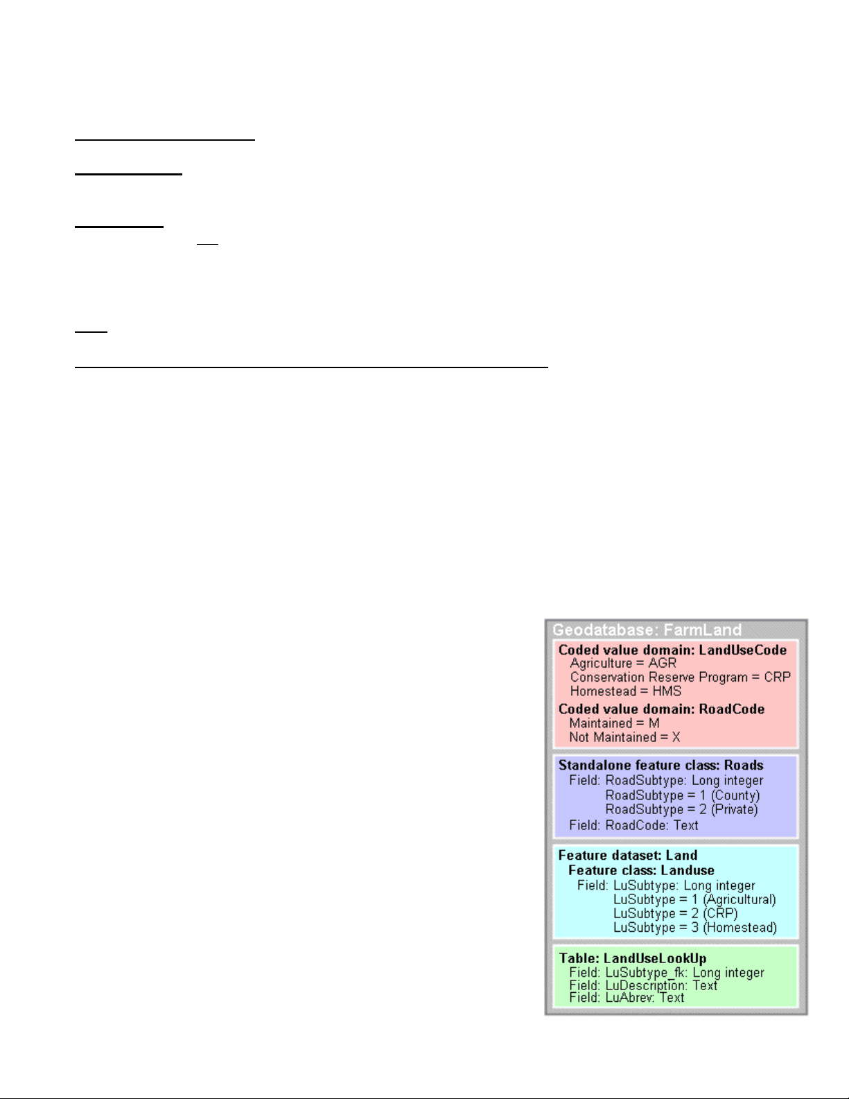
4. In ESRI’s ArcGIS terminology, a data model can be a type of a
diagram that illustrates the geodatabase design. The greatest
advantage of a data model is that the logical and relational decisions
of the database structure have already been performed. Specifically,
the FarmLand data model looks like the diagram to the right. It's not
important that you understand the specifics of the model right now.
What is important is that you recognize some of the database
structural elements depicted by the diagram. There are five objects in
this diagram: two coded value domains, a standalone feature class, a
feature dataset (with a single feature class), and a table. A ―coded
value domain‖ is a type of attribute domain that defines a set of
permissible values for an attribute in a geodatabase. Coded value
domains consist of a code and its equivalent value. In the FarmLand
data model, there are three coded value domains that the attribute
LandUseCode can carry: AGR, CRP, and HMS. There are two coded
value domains that the RoadCode attribute can carry: M and X.
Within the FarmLand data model is one standalone feature class,
Roads. This feature class consists of polylines that can be identified
by attributes as either 1 (County) or 2 (Private). In geodatabases, a
subset of features in a feature class or objects in a table that share
the same attributes is called a subtype. The feature dataset Land,
has one feature class Landuse. This feature class is composed of
polygon features that can carry three attributes. Finally, a
LandUseLookUp table is also a part of this data model.