Download Computing Paths in Alignment Graphs: Problem Solutions and more Assignments Computer Science in PDF only on Docsity!
Homework 1
Due: September 18, 8:30pm
Problem 1 (5 points)
- The complimentary sequence to the following string of nucleotides 5’- GCATATCGTAATGCCATA - 3’ is 3’- CGTATAGCATTACGGTAT - 5’, or more conventionally written as 5’- TATGGCATTACGATATGC - 3’.
- The mRNA sequence is the same as the coding strand, except that T’s are replaced by U’s. So it should be: 5’- GCAUAUCGUAAUGCCAUA - 3’.
- Each amino acid is coded by three nucleotides. By looking up the table of genetic code, we have: GCA UAU CGU AAU GCC AUA ⇒ Ala-Tyr-Arg-Asn-Ala-Ile
Problem 2 (15 points)
Starting point
(m, n)
destination
(i, j)
(i-1, j-1) (i-1, j)
(i, j-1)
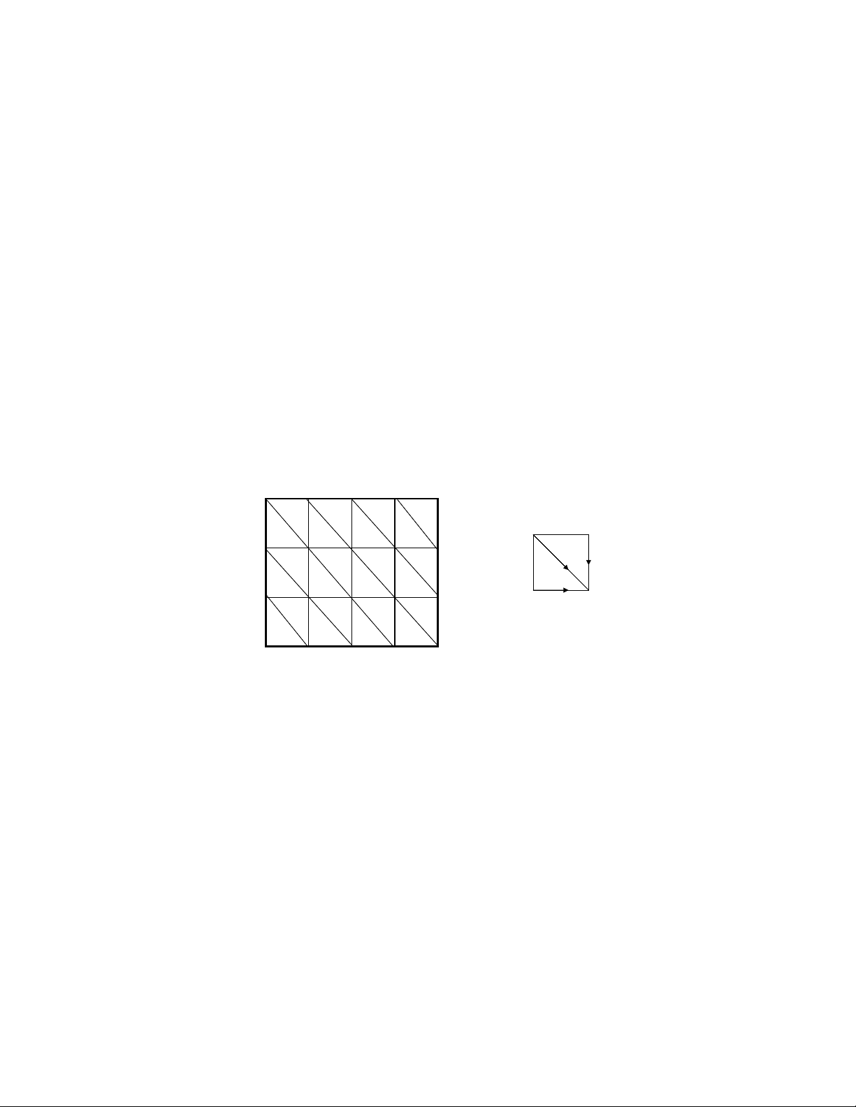
(1) The number of alignments between two sequences is the number of paths from the top left corner to the bottom right corner in the alignment graph, given certain restrictions on what is a legitimate move. For this problem, our next move does not depend on our previous move, i.e., we are free to take any direction at any time (not going backwards of course). Let each node be labeled by a two-tuple (i, j), where i and j are the row and column indices (both indices start from 0). Let F(i, j) be the number of paths from node (0, 0) to node (i, j). To get to (i, j), we may come from one of the three diretions: from (i-1, j-1) using a diagonal edge, from (i, j-1) using a horizontal edge, or from (i-1, j) using a vertical edge. (You may say that from (i-1, j-1) we can go to (i, j-1) first and then go to (i, j). But we will not count that, otherwise we are double-counting the paths using (i, j-1)). Therefore, the total number of paths from (0, 0) to (i, j) is simply the sum of the numbers of paths to the three neighboring nodes: (i-1, j-1), (i, j-1) and (i-1, j). The recursive definition of F(i, j) is straightforward:
F (i, j) = F (i − 1 , j − 1) + F (i, j − 1) + F (i − 1 , j) (1) (2) Given the recursive function, to compute the value for F(10, 10) is also simple. We can have a 11x matrix, and the value in the (i,j) cell corresponds to F(i, j) (here the row and column indices of the matrix also start from 0). We can gradually fill in the values, starting from F(0, 0). It is somewhat tricky to get the values for the first row and first column. It will be clear, however, if you remember the meaning of F(i, j): F(0, j) is the number of paths from (0, 0) to (0, j) in the alignment graph. There is only one way to get
to (0, j): from (0, 0) to (0, 1) to (0, 2), ..., to (0, j). So the value F(0, j) has to be 1 for all j. The same thing for F(i, 0). One last thing, however, is about the value F(0, 0). Should it be 0 or 1? Maybe you really cannot convince yourself. Fine. We can easily figure out the value for F(1, 1), which is the number of paths from (0, 0) to (1, 1). Apparently F(1,1) = 3. So we know F(0, 0) = 1 from Equation (1), although the value is not important any more for computing F(10, 10) after we know F(1,1). Now, given the values in the first row and first column, you can easily fill in the table using Equation (1). The table should look like this:
(3) The alignments between ab and xyz may have lengths 3, 4 or 5. There are three alignments of length 3: ab- xyz
a-b xyz , and -ab xyz
Now let’s enumerate all alignments of length 4: ab- - -xyz
ab- - x-yz
a-b- -xyz
a-b- xy-z
a- -b xyz-
a- -b -xyz
-ab- x-yz
-ab- xy-z
-a-b x-yz
-a-b xyz-
Finally the alignments of length 5: ab- - -
a-b- - -x-yz ,^
a- -b- -xy-z ,^
a- –b -xyz- ,^
-ab- - x- -yz ,^
-a-b- x-y-z ,^
-a- -b x-yz- ,^
- -ab- xy- -z ,^
- -a-b xy-z- ,^
- -ab xyz- -. Together, we have 3 + 12 + 10 = 25 alignments between ab and xyz. From the table above, we can see that indeed F(2,3) = 25.
Problem 3 (15 points)
(1) Here again the number of alignments between two sequences is the number of paths from the top left corner to the bottom right corner in the alignment graph. But there are certain restrictions on what is a legitimate move depending on our previous move. To get to (i, j), we may come free three directions: take a diagonal edge from (i-1, j-1), a vertical edge from (i-1, j), or a horizontal edge from (i, j-1). If we were from (i-1, j-1), that’s fine, we can always take the diagonal path. However, if we were from (i-1, j), the previous step must be a diagonal edge from (i-2, j-1) or a vertical edge from (i-2, j). Otherwise a path (i-1, j-1) - (i-1, j) - (i, j) constitutes an alternating gap. Similarly, if we were from (i, j-1), the previous step must be either a diagonal edge from (i-1, j-2), or a horizontal edge from (i, j-2). To calculate the number of paths to (i, j), we need two additional matrices. Let F(i, j) be the number of paths from (0, 0) to (i, j), with the constraints that no alternating gaps are allowed. Define G(i, j) as the number of paths from (0, 0) to (i, j), with the constraints that the last move is a diagonal or vertical edge, i.e., we are from (i-1, j-1) or (i-1, j) but not (i, j-1). Similarly, define H(i, j) as the number of paths from (0,
- to (i, j), with the constraints that the last move is a diagonal or horizontal edge, i.e., we come from (i-1, j-1) or (i, j-1), but not (i-1, j). Based on our reasoning above, F(i, j) can be computed recursively by:
F (i, j) = F (i − 1 , j − 1) + G(i − 1 , j) + H(i, j − 1). (2)
Problem 4 (20 points)
Your score distribution should look like the figures below. Your figures may be slightly differnet depending on how you have chosen your bins, but they should have similar shapes.
−20 −10 0 10 20
0
200
400
600
800
1000
1200
Alignment score
Number of sequences
Global alignment file1 vs file
−20 −10 0 10 20 30
0
200
400
600
800
1000
1200
Alignment score
Number of sequences
Global alignment file3 vs file
0 5 10 15 20 25
0
500
1000
1500
2000
Alignment score
Number of sequences
Local alignment file1 vs file
5 10 15 20 25
0
500
1000
1500
2000
Alignment score
Number of sequences
Local alignment file3 vs file
A few things you can observe from the figures. (1) The alignment scores between the sequences in file3 and file4 are higher than the alignment scores between the sequences in file1 and file2, for both global and local alignments. This is because the sequences in file3 and file4 have very high AT content. Therefore, the sequences in file3 and file4 may have a lot of A’s and T’s, and the alignment between the sequences in file3 and file4 may get high scores by chance. In fact, all the sequences here were randomly generated and do not contain any homology. Yet some of them consistently have higher alignment scores than the others. This shows that (a) it is necessary to take into account the base frequencies when designing substitution matrices (here we’ve used uniform scores for all matches, which may not be a good idea), and (b) we should estimate p-values for alignment scores instead of comparing raw scores. (2) The local alignment scores are higher than global alignment scores. In fact, if you had compared your local alignment scores and global alignment scores more carefully, you might have found that for any pair of sequences, the local alignment score is never lower than the global alignment score. This is easy to
understand: local alignment achieves a higher score by discarding some of the badly aligned flanking regions. If there is a global alignment with a higher score than local alignments, the Smith-Waterman algorithm will simply return the global alignment. (3) The local alignment score distribution is not symmetric, with a long tail on the right hand side, similar to the extremve value distribution (EVD). We know from lecture that ungapped local alignment scores follow EVD. Here we can see that gapped local alignment scores can also fit EVD nicely. In contrast, the global alignment scores seem to be symmetric and do not follow EVD.
Bonus (5 points)
You get this five points if you answered my survey questions :-).